사용 패키지
1. tensorflow 2.x
2. keras
3. numpy = 다차원 배열 처리
4. re = 필요없는 문자 제거
5. matplotlib = 그래프 표시
데이터셋 다운로드 및 데이터 로드
# 7.19 Naver Sentiment Movie Corpus v1.0 다운로드
path_to_train_file = tf.keras.utils.get_file('train.txt', 'https://raw.githubusercontent.com/e9t/nsmc/master/ratings_train.txt')
path_to_test_file = tf.keras.utils.get_file('test.txt', 'https://raw.githubusercontent.com/e9t/nsmc/master/ratings_test.txt')
# 7.20 데이터 로드 및 확인
# 데이터를 메모리에 불러옵니다. encoding 형식으로 utf-8 을 지정해야합니다.
train_text = open(path_to_train_file, 'rb').read().decode(encoding='utf-8')
test_text = open(path_to_test_file, 'rb').read().decode(encoding='utf-8')
# 텍스트가 총 몇 자인지 확인합니다.
print('Length of text: {} characters'.format(len(train_text)))
print('Length of text: {} characters'.format(len(test_text)))
print()
# 처음 300 자를 확인해봅니다.
print(train_text[:300])
학습을 위한 정답데이터(Y)
# 7.21 학습을 위한 정답 데이터(Y) 만들기
train_Y = np.array([[int(row.split('\t')[2])] for row in train_text.split('\n')[1:] if row.count('\t') > 0])
test_Y = np.array([[int(row.split('\t')[2])] for row in test_text.split('\n')[1:] if row.count('\t') > 0])
print(train_Y.shape, test_Y.shape)
print(train_Y[:5])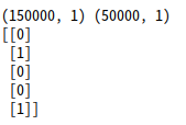
Train data의 입력(X)에 대한 1차 정제(Cleaning)
# 7.22 train 데이터의 입력(X)에 대한 정제(Cleaning)
import re
# From https://github.com/yoonkim/CNN_sentence/blob/master/process_data.py
def clean_str(string):
string = re.sub(r"[^가-힣A-Za-z0-9(),!?\'\`]", " ", string)
string = re.sub(r"\'s", " \'s", string)
string = re.sub(r"\'ve", " \'ve", string)
string = re.sub(r"n\'t", " n\'t", string)
string = re.sub(r"\'re", " \'re", string)
string = re.sub(r"\'d", " \'d", string)
string = re.sub(r"\'ll", " \'ll", string)
string = re.sub(r",", " , ", string)
string = re.sub(r"!", " ! ", string)
string = re.sub(r"\(", " \( ", string)
string = re.sub(r"\)", " \) ", string)
string = re.sub(r"\?", " \? ", string)
string = re.sub(r"\s{2,}", " ", string)
string = re.sub(r"\'{2,}", "\'", string)
string = re.sub(r"\'", "", string)
return string.lower()
train_text_X = [row.split('\t')[1] for row in train_text.split('\n')[1:] if row.count('\t') > 0]
train_text_X = [clean_str(sentence) for sentence in train_text_X]
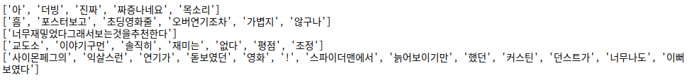
# 문장을 띄어쓰기 단위로 단어 분리
sentences = [sentence.split(' ') for sentence in train_text_X]
for i in range(5):
print(sentences[i])
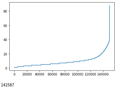
각 문장의 단어 길이 확인
import matplotlib.pyplot as plt
sentence_len = [len(sentence) for sentence in sentences]
sentence_len.sort()
plt.plot(sentence_len)
plt.show()

print(sum([int(l<=25) for l in sentence_len]))
단어 2차 정제 및 문장 길이 줄임
# 7.24 단어 정제 및 문장 길이 줄임
sentences_new = []
for sentence in sentences:
    sentences_new.append([word[:5] for word in sentence][:25])
sentences = sentences_new
for i in range(5):
    print(sentences[i])
Tokenizer와 pad_sequences를 사용한 문장 전처리 및 Tokenizer의 동작 확인
# 7.25 Tokenizer와 pad_sequences를 사용한 문장 전처리
from tensorflow.keras.preprocessing.text import Tokenizer
from tensorflow.keras.preprocessing.sequence import pad_sequences

tokenizer = Tokenizer(num_words=20000)
tokenizer.fit_on_texts(sentences)
train_X = tokenizer.texts_to_sequences(sentences)
train_X = pad_sequences(train_X, padding='post')

print(train_X[:5])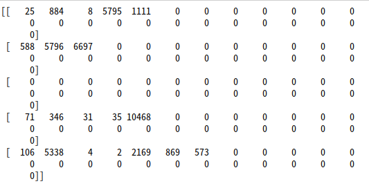
# 7.26 Tokenizer의 동작 확인
print(tokenizer.index_word[19999])
print(tokenizer.index_word[20000])
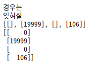
temp = tokenizer.texts_to_sequences(['#$#$#', '경우는', '잊혀질', '연기가'])
print(temp)
temp = pad_sequences(temp, padding='post')
print(temp)
Tokenizer와 pad_sequences를 간략히 설명드리면
- Tokenizer
1. text를 나누는 단위를 토큰(token)이라고 하고, 텍스트를 토큰으로 나누는 작업을 토큰화(tokenization)이라고 함
2. 텍스트 데이터에 토큰화를 적용하고, 수치형 벡터에 연결하는 작업을 하는 것을 tokenizer라고 함
- pad_sequences
1. 배열과 같이 길이가 있는 데이터에서 길이가 같지않고 적거나 많을 때 일정한 길이로 맞춰주는 라이브러리
2. 1차원, 2차원, 3차원 데이터 모두 사용이 가능함
7.27 감성 분석을 위한 모델 정의
여기서 LSTM으로 되어있는 부분을 SimpleRNN, GRU로 코드를 수정해서 학습을 진행하면 됩니다.
# 7.27 감성 분석을 위한 모델 정의
model = tf.keras.Sequential([
    tf.keras.layers.Embedding(20000, 300, input_length=25),
    tf.keras.layers.LSTM(units=100),
    tf.keras.layers.Dense(2, activation='softmax')
])

model.compile(optimizer='adam', loss='sparse_categorical_crossentropy', metrics=['accuracy'])
#sgd = optimizers.SGD(lr=0.01, decay=1e-6, momentum=0.9, nesterov=True)
#model.compile(optimizer='adam', loss='categorical_crossentropy', metrics=['accuracy'])
model.summary()
영화감상평 분석 모델 학습
-> 5번만 학습해도 잘나오지만 학습횟수는 자유입니다. 오히려 학습횟수가 많아질수록 학습데이터는 loss가 줄어들겠지만 val데이터나 test데이터에서 심하게 과적합 될 가능성이 높아지므로 추천은 안드립니다.
# 7.28 감성 분석 모델 학습
history = model.fit(train_X, train_Y, epochs=5, batch_size=128, validation_split=0.2)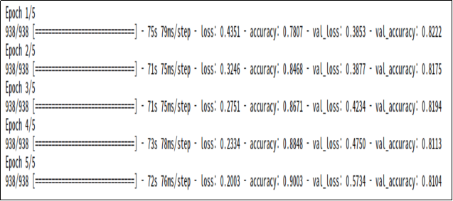
감성 분석 모델 학습 결과 확인
# 7.29 감성 분석 모델 학습 결과 확인
import matplotlib.pyplot as plt
plt.figure(figsize=(12, 4))

plt.subplot(1, 2, 1)
plt.plot(history.history['loss'], 'b-', label='loss')
plt.plot(history.history['val_loss'], 'r--', label='val_loss')
plt.xlabel('Epoch')
plt.legend()

plt.subplot(1, 2, 2)
plt.plot(history.history['accuracy'], 'g-', label='accuracy')
plt.plot(history.history['val_accuracy'], 'k--', label='val_accuracy')
plt.xlabel('Epoch')
plt.ylim(0.7, 1)
plt.legend()

plt.show()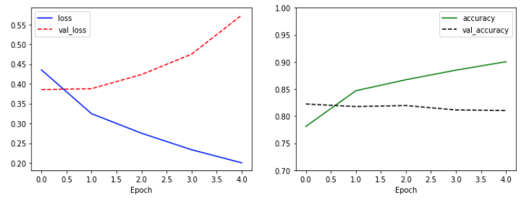
테스트 데이터 평가
# 7.30 테스트 데이터 평가
test_text_X = [row.split('\t')[1] for row in test_text.split('\n')[1:] if row.count('\t') > 0]
test_text_X = [clean_str(sentence) for sentence in test_text_X]
sentences = [sentence.split(' ') for sentence in test_text_X]
sentences_new = []
for sentence in sentences:
    sentences_new.append([word[:5] for word in sentence][:25])
sentences = sentences_new

test_X = tokenizer.texts_to_sequences(sentences)
test_X = pad_sequences(test_X, padding='post')

model.evaluate(test_X, test_Y, verbose=0)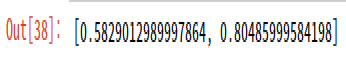
데이터셋의 문제로 과적합현상이 발생되었지만 최종결과에서는 크게 영향이 없었습니다.
여기서 과적합이란?
overfitting(과적합)은 학습 데이타를 과하게 학습하는 것을 뜻 함, 학습 데이타는 실제 데이타의 부분 집합이므로 학습데이타에 대해서는 오차가 감소하지만 실제 데이타에 대해서는 오차가 증가하는 현상을 말합니다.
임의의 문장 감성 분석 결과 확인
# 7.31 임의의 문장 감성 분석 결과 확인
test_sentence = '재미있을 줄 알았는데 완전 실망했다. 너무 졸리고 돈이 아까웠다.'
#test_sentence = '사이몬페그의 익살스런 연기가 돋보였던 영화!스파이더맨에서 늙어보이기만 했던 커스틴 던스트가 너무나도 이뻐보였다'
test_sentence = test_sentence.split(' ')
test_sentences = []
now_sentence = []
for word in test_sentence:
    now_sentence.append(word)
    test_sentences.append(now_sentence[:])

test_X_1 = tokenizer.texts_to_sequences(test_sentences)
test_X_1 = pad_sequences(test_X_1, padding='post', maxlen=25)
prediction = model.predict(test_X_1)
for idx, sentence in enumerate(test_sentences):
    print(sentence)
    print(prediction[idx])
문장평가는 처음에 제시한 예제를 실행했습니다.
최종결과는 LSTM의 경우 부정이 99.8퍼가 나오게 되었습니다.
이제 SimpleRNN 과 GRU를 똑같이 진행해서 나온 결과를 보면

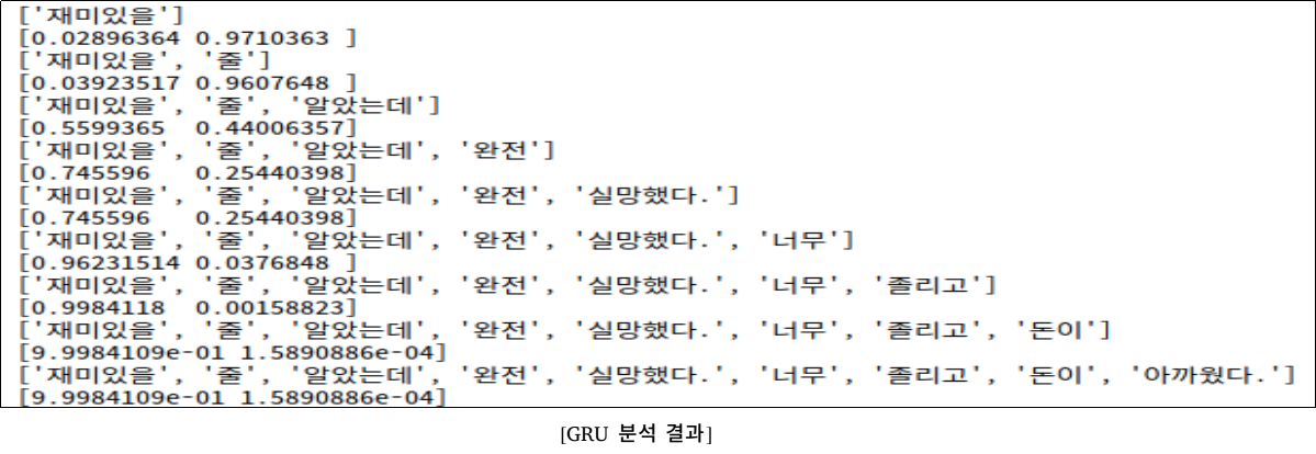
3모델을 비교분석한 결과 GRU가 가장 99.9퍼로 잘나왔고 LSTM, SimpleRNN 순으로 성능이 나왔습니다.
GRU의 경우는 일정경우에만 LSTM보다 뛰어나다고 하는데 그 일정경우에 대해서는 조사하지 못했습니다.
참고 깃헙
wikibook/tf2
《시작하세요! 텐서플로 2.0 프로그래밍》 예제 코드. Contribute to wikibook/tf2 development by creating an account on GitHub.
github.com
본 코드는『시작하세요! 텐서플로 2.0 프로그래밍』 예제 코드를 이용하여 작성되었습니다.
'인공지능 > 실습' 카테고리의 다른 글
| [pytorch]pytorch를 이용한 stylegan2 ada 실습 (0) | 2021.02.05 |
|---|---|
| [KNN-python]KNN을 이용한 시계열 분류 (0) | 2021.02.01 |
| [LSTM]을 이용해서 삼성전자 주식 예측해보기 (0) | 2020.12.01 |
| [tensorflow GAN]tensorflow GAN(심층 합성곱 생성적 적대 신경망) 기본예제 (0) | 2020.11.26 |
| [tensorflow GAN]인공지능 뷰티간(BeautyGAN) 모델을 이용해서 생얼 화장시키기 (0) | 2020.11.24 |